COMP 150 Class Notes

These notes are basically for everything except the Hands-on Python Tutorial.  That is a free-standing unit that we take up after the Course Introduction, see the Course Schedule for dates. 

Videos for most of the sections below are in the beyondPython folder in GoogleDocs, discussed in the Resources.

Sections that correspond to the start of a video have (vid) at the end of the title.

Table of Contents

1. Course Introduction
1. Computer Science Areas
2. Introductory Approaches
3. Past Final Projects (vid)
4. Using the Hands-on Python Tutorial
   
2. After Python and Underneath Python (vid)
3. Binary Arithmetic  (vid)
   1. Converting binary to decimal numerals
   2. Converting decimal to binary numerals (vid)
   3. Hexadecimal (Base 16) (vid)
      
   4. Converting Binary to Hexadecimal
   5. Hexadecimal to Binary
   6. Formatting Binary, Octal, and Hexadecimal in Python
4. Pip Assembler (vid)
   1. Pip Assembler Simulator (vid)
      
   2. An Introduction to Pip Machine Language (vid)
      
   3. More on the Simulator and Pip (vid)
   4. Format of my Pip assembler
   5. Assignment Translation Applet Introduction (vid)
      
   6. Loops and Symbolic Address Labels (vid)
   7. Practice Using jumps (vid)
      
   8. Translation Between Machine Language and Assembler (vid)
5. Boolean Algebra, Truth Tables, and Digital Circuits (vid)
   1. Boolean Algebra and Truth Tables (vid)
   2. Rules of Boolean Algebra (vid)
   3. Transistors, Gates, and Circuits (vid)
   4. Gates Applet (vid)
      
   5. Finding a Boolean Expression for a truth table (vid)
   6. Computer Addition (vid)
   7. Mutiplexers (vid)
   8. Latch Circuit (vid)
   9. Chip Fabrication (vid)
6. Conclusion

Course Introduction

Computer Science Areas

Computer Science centers on algorithms:  unambiguous, step by step instructions for how to accomplish a particular task in a finite amount of time.

Peter J. Denning lists seven main categories in computing

• Computation (meaning and limits of computation)

• Communication (reliable data transmission)
  

• Coordination (cooperation among networked entities)

• Recollection (storage and retrieval of information)

• Automation (meaning and limits of automation)

• Evaluation (performance prediction and capacity planning)

• Design (building reliable software systems)

Introductory Approaches

 With all there many aspects, college introductions have handled things differently over time:

1. Historically students usually started with several heavy programming courses before anything else, giving little initial idea of all the other parts of computer science!

2. Then there was a reaction to breadth-first, essentially no programming.  This is partly because in the past popular languages had a steep learning curve.  Instead of much programming in a real computer language, breadth-first courses have brought algorithms written in English to a central place.

3. That brings us to the present with this course.  Programming is important, and now there is an excellent recent language Python:  extremely simple to learn and understand (close to English) and very powerful  - why do much in English outlines when with about as much work you can demonstrate things on the computer using Python?  Plus, even beginners can write programs to simplify their own personal tasks.  Hence we spend a fair amount of our time on algorithms actually working with Python. We still keep the idea that Computer Science is much more than programming, and look at history, applications, and their relationship to the WWW.  We dig down into the guts of a computer below what we see from the high-level language Python, to machine language and assembler code, and to the hardware underneath.  We look beyond Python to application areas like graphics and web servers.

In an introductory course we cannot cover a whole lot with any depth, but we will deal at some level with all the areas:  We will think about what we can compute.  The last part of the section using Python will involve communication and cooperation between web client and server.  We introduce a basic way to store information, in files.   We will design, write and evaluate programs to automate the solution of problems.

For the programming in Python, we use custom tutorials written by Dr. Harrington,  Hands-on Python Tutorial.  For the other areas, Dr. Harrington has written these online notes that you are reading.     

We are not alone in choosing Python:  Much of the control of Google is by Python (about 1/3 of the code they write for their own applications, plus the Google App Engine providing free web sites to anyone requires writing Python code), as is much of the administration of Unix.  Much scientific programming is done in Python.  Microsoft now has a Python, too, for its own .net platform.  Python is freely available for Windows, modern Macs, and Linux.

Past Final Projects (vid N1D)

Further instructions (for Windows):

1. Save the file. In a Loyola Windows lab use d:\Userdata
2. Find that place in the file system, for instance via My Computer, or your browser may have an Open Enclosing Folder option.
3. Right click on pastGames.zip,
4. Select Extract All....
5. Follow the default choices
6. When the new directory pops up, double click on Python program hole or asteroids
7. Play! Try the other game.

Using the Hands-on Python Tutorial

Python topics are covered in the Hands-on Python Tutorial.  Homework exercise links and topic timing are in the Course Schedule.

While the tutorial introduces all the topics, there is more to say about using it effectively.  There is way too much detail to just obsorb all at once,  So what are the first things to learn? 

More imprtant than memorizing details is having an idea of the building blocks available and how they are useful.  For the most direct exercises, you might  just look back over the most recent section looking for related things, but that will not work when you have scores of sections that might have useful parts!  The basic idea of the building blocks should be in your head. For instance, after going in the Tutorial through 1.10.4, you will want to have very present:

• You can use numbers and do arithmetic.
• You can store and retrieve data using variable names and assignment statements.
• Python has many useful built-in functions that can affect the system or return results for you to use.
  
• You can get keyboard input from the user and print things back for the user.
• Data comes in different types, and you can convert where it makes sense.
• You can use strings and generate them in many ways:  literal strings, addition operator (+), string format method.

After Python and Underneath It (vid N2)

We have seen how we can tell the computer what to do with the fairly simple syntax of Python.  The course started there because it was relatively easy place to accomplish a lot.  As you were introduced to it, Python was just given to you.  We could immeditately see, experimenting in the Shell, that Python worked on your computer.  But how?  Python operates on the top of many layers of computer hardware and software.  We are going to take an introductory exploration down into the hardware and logic of computers.  Here is an outline of that path:

Machine Language and Assembler:  Next we work with the instructions that are part of the computer's hardware.  To be feasible in hardware, the instructions need to be rather simple.  They are the machine language of a particular computer. We will look at machine language (actually an extra simple model of a machine language), mostly though its more human friendly variant, assembler.  We see how higher level ideas we express in languages like Python can be translated into and implemented with a very limited group of simple instructions.  The Python interpreter does this conversion for Python programs.

Boolean Logic and Circuits:  Once we have an idea of how simple instructions can be combined to implement high level programs, the final stage is to look at how hardware can implement individual instructions.  In Python we built up logical expressons with and, or, and not.  We will look much more systematically at logical expressions, and see how they relate to circuits and machine language instructions. 

Binary Arithmetic  (vid N3A)

Computers depend on arithmetic and numerical codes, and the simplest way to do arithmetic in an electronic computer is with base 2, the binary number system.  First review our usual decimal system, in powers of 10:

place value - powers of 10, base 10 (recall anything to the 0 power is 1)
3072 = 3*10³ + 0*10² + 7*10¹ + 2*10⁰
This is easiest to write out from right to left, so you start counting powers from 0).  Note that we also need symbols for the numbers less than ten (0-9)
We think of 3072 as a number.  In this discussion that is too sloppy:  The symbolism is a numeral representing a number.
Another representation could be a pile of 3072 counters, or a Roman numeral MMMLXXII.  

Also we can make different numerals by using a different base, in particular the simplest one, and the one used in computers hardware:

Converting binary to decimal numerals

(included in previous video)  Binary (base 2) uses powers of 2 for place value and two symbols 0, 1, for the numbers less than 2:
I will use a subscript to indicate the different base:  11011₂ means the base 2 numeral 11011:  If we expand the powers explicitly from the right, in normal arithmetic, this means:
1*2⁴ + 1*2³ + 0*2² + 1*2¹ + 1*2⁰
= 16 + 8 + 2 + 1 = 27₁₀. 
The base 10 numeral 27 refers to the same number as the base 2 numeral 11011.

For base 2, where the only coefficients are 0 and 1, a shorthand for converting small base 2 numerals to decimal is to think of the sequence of the possible powers of 2, and then just add in the values where there is a 1 in the base 2 numeral:

Looking ahead, download pipFiles.zip, and unzip it on your computer or on your flash drive.  The pipFiles directory also contains an Idle shortcut and a module for studying bases, bases.py.  To follow along for now, open Idle in this directory.

Binary to decimal conversion is done directly by Python.  Try the following in the Python Shell, stopping without a close parenthesis, and look at the popup window in the Python shell, pointing out possible parameters:

int('11011'

int('11011', 2)

Converting decimal to binary numerals (vid N3B)

Now we go in the other direction:  finding the binary place values from a given integer number:
Suppose we have an unknown int, i, which can be represented as a 4 digit decimal.  How could we recover the digits by doing simple arithmetic?  (On a computer, there is something to do here, since the number is actually stored in a binary form.)  A small amount of algebra can show us the general approach:  For the algebra we name the 4 digits, say p, q, r, s, then we have
i = p*10³ + q*10² + r*10¹ + s
Note all but the last term are divisible by 10, so
s = i % 10
We have s, so we can remove it from our power sequence with integer division by 10. Change i so
i = i//10 =  p*10² + q*10¹ + r
Now use the same trick to recover r!  
r = i % 10
Continue, let
i = i//10 = p*10¹ + q
q = i % 10
One more time, let
i = i//10 = p
p = i % 10
To illustrate the general algorithm we can go through one more step:  Let 
i = i//10 = 0 - - getting  a 0 result means we are done.

This can turn into a general algorithm in Python:

def decimal(i):
 """return a string of decimal digits representing 
 the nonnegative integer i."""
 if i == 0:
 return "0"
 numeral = ""
 while i != 0:
 digit = i % 10
 numeral = str(digit) + numeral # add next digit on the LEFT
 i = i//10
 return numeral

Decimal to binary conversion:  same idea as for digits of unknown number, but generate base is 2, not 10:

def toBinary(i):
 """return a string of binary bits representing 
 the nonnegative integer i."""
 if i == 0:
 return "0"
 numeral = ""
 while i != 0:
 digit = i % 2
 numeral = str(digit) + numeral # add next digit on the LEFT
 i = i//2
 return numeral

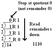
For illustration, this can also be done by hand.  To convert 14₁₀ to 1110₂, start with 14 (at the bottom of the picture) and repeatedly divide by 2 until you get a 0 quotient:
 
Binary is verbose!  We will see that there is a very simple relationship between base 2 and base 16 = 2⁴.  Base 16 takes up about a quarter of the space of base 2, and so it is used in many places to communicate binary information compactly.  

Hexadecimal (Base 16) (vid N3C-E)

We have not discussed bases above 10 yet.   Problem:  We need 16 distinct one-character symbols for 0 through 15.  You run out of symbols using  normal digits at 9. Solution: then start with letters, so decimal 10 corresponds to hexadecimal A, 11->B, 12->C, 13->D, 14->E, 15->F.  The following table for 0-15 decimal has columns for  hexadecimal and also binary.  We will find the binary useful shortly:

The base 16 numeral 2A8C  can be expressed as a sum of terms for different powers of 16.  To express this in terms of normal base 10 numerals,  you have to also convert individual digits.  In particular hexadecimal A means decimal 10 and hexadecimal C means decimal 12. The full expansion, with powers increasing from the right, is

so using the explicit base subscripts, 2A8C₁₆ = 10892₁₀.

In Python the conversion of a number 0 through 15 to a hexadecimal digit character can be expressed many ways.  One clear approach is:

def digitChar(n):
 '''return single character for digits with decimal value 0 through 15'''
 if n < 10:
 return str(n)
 if n == 10:
 return 'A'
 if n == 11:
 return 'B'
 if n == 12:
 return 'C'
 if n == 13:
 return 'D'
 if n == 14:
 return 'E'
 if n == 15:
   return 'F'

Notice that the digitChar function trivially produces the right digit for any number 0, 1, 2, ... 9.  

The conversion above from decimal  to base 2 and 10 using division and remainders are very similar, except for division by the right base.  We can make a more general function that will work with any base 2 through 16:

def intToBase(i, base):
 """Return a string representing the nonnegative integer i
 in the specified base, from 2 to 16."""
 i = int(i) # if i is a string, convert to int
 if i == 0:
 return '0'
 numeral = ""
 while i != 0:
 digit = i % base
 numeral = digitChar(digit) + numeral # add next digit on LEFT
 i = i//base
 return numeral

There is one further change in intToBase to accommodate bases from 11 through 16:  Instead of creating a digit character with just str(digit), digitChar(digit)is needed, as defined above.  

The intToBase function and several others are include in bases.py in pipFiles.zip file referenced earlier.  It sits in the examples directory for the course (not in the Python tutorial examples). 

Understanding hexadecimal allows interpretation of colors in web pages or in Python graphics.  The Python graphics module has the color_rgb function to generate custom colors based on values for the red, green and blue components in the range 0 to 255. See the documentation. Integers in this range can be described by a two place hexadecimal  numeral.  Look at  what the color_rgb  function actually produces in the Python Shell:

>>> from graphics import color_rgb
>>> color_rgb(255, 35, 0)
'#ff2300'

After the marker '#' that indicates the color is not a predefined color name, you see the hexadecimal for each color component, ff, 23, and 00. The same system of '#' followed by six hexadecimal characters is used in html source attributes, so you can see and manipulate custom colors in html, too.

Now back to the easy conversions between binary and hexadecimal, mentioned earlier.  

Converting Binary to Hexadecimal

The basic idea is to convert each 4 bits of a binary numeral to a single hexadecimal character. In detail:
Group the binary digits in 4's, starting from the right.  Example:

A bigger example:

Now the reverse process:

Hexadecimal to Binary

See bases.py in the examples directory for the course.  The hexToBin and binToHex functions manipulate pieces of strings and use some of the string methods and string indexing syntax from Chapter 2 of the Hands-on Python Tutorial.

If you do not want to do any arithmetic in converting between binary and hexadecimal, you can use the decimal/hex/binary table above or run the table() function in bases.py to produce:

Dec Hex Bin
 0 0 0000
 1 1 0001
 2 2 0010
 3 3 0011
 4 4 0100
 5 5 0101
 6 6 0110
 7 7 0111
 8 8 1000
 9 9 1001
 10 A 1010
 11 B 1011
 12 C 1100
 13 D 1101
 14 E 1110
 15 F 1111

Instant converter applets at http://www.easycalculation.com/hex-converter.php

The same idea works for conversion between binary and base 8, octal.  Octal is used to express some Unix/Linux 3-bit permission codes.  

Formatting Binary, Octal, and Hexadecimal in Python

This section relates recent ideas to previous Python work, but it is not central to the current ideas.  It is useful for testing simple results you work on by hand, like those in the next section.

You can generate hexadecimal, octal, and binary numerals in format strings in Python using format specifiers 'X', 'o', and 'b'  (letter o, for octal, not the number 0).  Like the syntax for float formatting, the base formatting may be used in the format function or after a colon inside braces in the string format method:

>>> 'binary:', format(27, 'b')
'binary: 11011'
>>> 'decimal: {0}, hex: {0:X}, octal: {0:o}, binary: {0:b}'.format(27)
'decimal: 27, hex: 1B, octal: 33, binary: 11011'

Also Python recognizes binary, octal, and hexadecimal numeric literals.  The literals start with 0 followed by the specifiers b, o (letter o), or X, and then digits appropriate for the base. 

>>> 0b11011
27
>>> 0X1B
27

The built-in functions hex, oct, and bin generate strings with these notations:

>>> bin(27)
'0b11011'
>>> hex(27)
'0x1b'

Sample Binary/Hexadecimal Converson Problems

Conversions to do by hand to check understanding:   (You can confirm with Python.) 

1. 10111 binary to decimal
2. 87 decimal to binary
3. 10011011011 binary to hexadecimal (short way)
4. 3AF hexadeciml to binary (short way)
5. Python/html graphics color '#a150ff' would be returned by what call to the color_rgb function with decimal number parameters?
   

Pip Assembler (vid N4)

As the beginning of the Hands-on Tutorial indicated, computer hardware does not execute Python directly.  Python and other high level languages must be converted to the very simple set of instructions that are directly built into the computer hardware, the machine language.  This is the first place we look underneath high level languages.

As we will see more in the gates unit, the state inside a computer is usually electrical, and the most dependable system uses voltages, either high or 0 (grounded) .  This means two possibilities.  This is a bit of information, the smallest possible amount.  We will arbitrarily refer to the two states as 0 and 1.  This is convenient for the binary number system!

Computers have a Central Processing Unit (CPU) connected by wires to a memory unit.  Operations take place inside the CPU, with some data maybe transferred in from memory or sent back to memory (and also external devices, though we will skip that part in our simple model).

Like in a Python string or list, memory is referenced by integer locations, 0, 1, 2, ....  There are several design decisions:  one is how much data to put in a single memory cell that can be individually referenced.  A common unit is a byte = 8 bits.  Pip uses a byte, as do the common processors used in Windows machines (and the latest Macs).  While a bit has two possible states, a byte has 2⁸ = 256 states.  Another choice is how big to allow memory to be.  So that one byte can used to refer to any cell in  the memory or our simulated machine, we will assume memory consists of no more than 256 cells (a very limited machine!).

A concept encouraged by Von Neumann in the 1940's was to encode the instructions as a form of data in the computer.  Before this approach, changing the program in a computer involved physically rewiring the computer!  With Von Neumann's approach, an instruction would be represented as a number in the computer's memory.  Hence an instruction must be a sequence of 0's and 1's, like

00010100 00000100  

I introduce the space in the middle only to delineate individual bytes.    

Since accessing memory is slower than internal operations in the CPU, all CPU's have places for special data to be stored inside of them.  One is an Instruction Pointer (IP), saying where in memory the next instruction starts.  CPU's also have one or more fast temporary data storage locations, called registers.  I follow the simple example in a text we used to use, the Analytical Engine, which has a single such location, called the Accumulator or Acc for short, that holds a byte of information, just like a memory cell.  

Pip Assembler Simulator (vid N4A)

For a simple conceptual view, look at the Pip Assembler simulator in the class web examples.  All files are included in pipFiles.zip.  

The zip archive contains the files needed for the Pip Assembler Simulator:  pipGUI.py, pipText.py, pip.py, pipHelp.py, hexBin.py, and sample program files,  simple.bin, simple.asm, arith.asm, sum2n.asm, ifElse.asm, etc.  

The main program is pipGUI.py.  Depending on how Python was installed on your particular computer, you might be able to run it from the operating system by just double clicking on it in the file window. If that doesn't work, you can also open the file and run it in IDLE.

You will see a graphical Window.  Click on the purple button that says BINARY, to see its 'native' state.  Look at the window as its various parts are described:

The state of the simulated computer is shown in the CPU (lower left) with its accumulator (Acc) and Instruction Pointer (IP).  The middle blue and right yellow blocks display memory.  

First focus on the big middle blue rectangle labeled CODE.  Instruction code in Pip is placed at the beginning of memory.  Each instruction takes up two bytes, so for convenience bytes are shown in pairs down the right portion of the main blue rectangle.   We will need to keep track of the locations of these instructions, so the left column in the  blue rectangle shows the address (in decimal) of the beginning of each instruction.  Beside the decimal address label is the same address in binary.  Because each instruction is two bytes, the address labels advance by 2's.

Now look at the right yellow rectangle labeled DATA.  For simplicity of display, we arbitrarily assume that the data for program variables is stored in the second half of memory, starting at address 128.  Each individual byte is a separate piece of data, so we show only one per line, at the right.  For our simple programs we will never need more than 8 variables, so only eight locations are displayed.  As in the code section, address labels in decimal and binary are shown.

The remaining parts of the display are for controlling the simulator.  They do not correspond to parts of Pip.  The left column of buttons and text boxes is labeled COMMANDS.  You should have already clicked on the command button labeled BINARY. 

 Let us load a machine language program into Pip. Make sure you have downloaded simple.bin.  You can open it in the Idle editor, to see the file format, if you like.  It contains five binary instructions.  

Type simple.bin into the Filename text box.  Then click LOAD.  The contents of the file appear as the first five instructions in Pip.

An Introduction to Pip Machine Language (vid N4B)

All Pip instructions use the Accumulator.  It is always a source of data and/or the destination of a result.  There are two other ways Pip refers to data.  One is to have the actual data encoded as the second byte of the instruction.  The more common way is to refer to a location in memory.  In this case the second byte is interpreted as the address in memory where the data resides.   That explains the second byte, so now the first byte.  It can be logically split into two four bit fields, for example

0001 0100 00000100  

In Pip we will have fewer than 16 basic operations, which are encoded in the second four bits.  

0001 0100 00000100  

The 0100 of this example means load a value into the accumulator.  We must distinguish where to get the value from, either the second byte of the instruction or a specified address in memory.  The first 4 bits (actually only 1 bit is needed) determine this.  The code is that 0000 means a memory address and 0001 means the actual data is in the second byte of the instruction.  That latter is the case above, where the second byte is 00000100 or 4 in decimal, so the full meaning of the instruction is load the value in the second byte (4) into the accumulator.

Look at the Simulator screen.  See that the accumulator (ACC) has a value of 0.  The instruction pointer (IP) shows the next instruction to execute.  It is also 0.  If you look at address 0 in the simulator you see the instruction we have been discussing.  Also note that the binary version of the address 0 in the code it highlighted in orange.  To more easily follow what is going on, it will always match IP.  Click STEP.   IP and the corresponding highlight should advance to 2, and the value in the accumulator should become 00000100 (or 4 in decimal).

One more machine language instruction, the one at address 2:

00000101 10000000    

or to look at the parts:

0000 0101 10000000    

The second four bits 0101 determine the type of instruction.  In this case it is "store the contents of the accumulator to an address in memory".  The second byte gives the address 10000000 (or 128 decimal).  For the Store instruction the second byte only makes sense as an address in memory, and the first four bits of the instruction, 0000, reflect this.   Hence the full instruction says to store the accumulator value at memory location 128.

Click STEP again.  Look at memory location 128 (or 10000000 in binary).  Also note IP in the CPU.

We could continue, but this gets tedious.  Reading this binary is a pain.  One of the first programs people wrote was an assembler, which translates something a bit more human readable into this binary code.  In the assembler written for this machine, the first two instructions discussed could be written

LOD #4
STO 128

Still not English or as close as Python but closer!  In place of the second four bit pattern we have a three letter mnemonic.  LOD is close to LOAD.  STO is the beginning of STORE.  The pound sign is sometimes used to mean 'number'.  The first instruction says to load the number 4.  The second instruction does not have the '#'.  This means the other interpretation of the second byte is used:  it refers to a memory location.  Be mindful of the presence or absence of '#'!  It is easy to make a mistake.

Click the button NONE under commands.  Now you see the instructions stated in assembler and all the address labels in decimal.

We will come back to machine language briefly at the end of our discussion of this simple CPU, but for the most part we will code things in assembler.

The next instruction is LOD #3.  From the earlier examples you should be able to figure out what that does.  Click STEP to check.  The next instruction is ADD 128.  It should be no surprise that this involves addition, and from the format you should see that it involves memory location 128.  We need two things to add.  Memory location 128 is one obvious operand.  The accumulator is also available. So the instruction adds the accumulator and memory location 128.  The final issue is where to put the result.  Fancier CPU's than Pip have more options, but in Pip all results go to the accumulator, except in the STOre instruction where a value is copied FROM the accumulator.  Hence the sum of the accumulator and memory location 128 are stored back into the accumulator.

Click STEP to check.

You can put the result of an addition or any other operation into memory:  It just takes an extra step.  Guess what the next instruction STO 129 does.  Click STEP and check.

Next is the HLT instruction, short for HALT.  Click STEP and the program stops (indicated on the screen by '- -' as the instruction pointer.

Click INIT.  This resets IP and ACC to 0.  You could step through the program again, or to see the result, just click RUN, and it goes (up to 100 steps) to the end.

In Python and other higher level languages we also store data in memory.  We refer to the data by name, not number.  Using names is easier.  The assembler can also handle that.  Click the button DATA under labels. Every place we had address 128 before, we now have W, and every place we had address 129, we now have X.  In this case the machine code was disassembled (from machine code to assembler code).  The machine code did not include names, so the simulator fakes it, and always uses the names you see in the DATA section labels, W, X, Y, Z, T1-4.  (These names have no particular significance:  they are the names used by  the old Analytical Engine.)  If you load a file with variable names, including ones different than W, X, ..., then pipGUI remembers them and uses them instead.  (The only restriction for the display is that they cannot be more than 8 characters long.)  In Python, variable names always are linked to data in memory.  In the Pip Assembler Simulator, the relationship is very simple and graphic!

More on the Simulator and Pip (vid N4C)

Click HELP.  See the message at the bottom.  This gives context sensitive help.  First click on HELP again for a summary.  This shows all the help for the simulator operations.  Return to here if you have questions.  It covers the command buttons, the comment area at the bottom, the close button, and it mentions how to get an assembler summary:  

Click the HELP button and then click in the blue CODE area.  Try that now.  For reference, the contents of this window are shown below:

Pip Assembler Summary
 Symbols Used
 X for a symbolic or numeric data address.
 #N for a literal number N as data
 Acc refers to the accumulator
 L refers to a symbolic code label or numeric code address
 Instructions Pseudo Python syntax for what happens
 Data Flow
 LOD X (or #N) Acc = X (or N)
 STO X X = Acc (copy Acc to location X)
 Control
 JMP L IP = L (go to instruction L)
 JMZ L if Acc==0: IP = L else: IP = IP+2 (normal)
 NOP No operation; just go to next instruction
 HLT Halt execution
 Arithmetic-Logic
 ADD X (or #N) Acc = Acc + X (or N)
 SUB X (or #N) Acc = Acc - X (or N)
 MUL X (or #N) Acc = Acc * X (or N)
 DIV X (or #N) Acc = Acc / X (or N)
 AND X (or #N) if Acc != 0 and X != 0: Acc=1 else: Acc=0
 NOT if Acc == 0: Acc = 1 else: Acc = 0
 CPZ X if X == 0: Acc = 1 else: Acc = 0
 CPL X if X < 0: Acc = 1 else: Acc = 0
 In source files: An instruction may be preceded by a label
 and a colon. Any line may end with a comment. A comment
 starts with ';' and extend to the end of the line.

We will gradually introduce the 14 instructions and the assembler syntax conventions.

Format of My Pip Assembler (vid N4D)

See arith.asm from the pipFiles:
 
  LOD #7   ; acc = 7   initialize variables
  STO W    ; W = acc  
  LOD #3   ; acc = 3
  STO X    ; X = acc  
  LOD #6   ; acc = 8
  STO Y    ; Y = acc
 
           ; Z = (W + X) * Y / 2
  LOD W    ; acc = W    
  ADD X    ; acc = acc + X ( = W+X )         
  MUL Y    ; acc = acc * Y ( = (W+X)*Y )    
  DIV #2   ; acc = acc/2 ( = (W+X)*Y/2 )              
  STO Z    ; Z = acc  ( = (W+X)*Y/2 )
  HLT      

Human comments are allowed starting with a ';' (same idea as the '#' in Python, but # is already used in Pip assembler.)  In the example the comments are a very direct translation into pseudo Python.  I use symbolic data names. 

Load arith.asm into pipGUI by typing in the name under filename, and clicking LOAD.  You should see the code, minus comments.  

If you switch your view to the text console (what would appear in the Python Shell  in Idle) at any point, you will see that the computer is showing you the results of playing computer:  A full history is kept.  (I will expect you to show your understand sequences of Pip instructions by playing computer, and this text history shows you exactly what you should be able to generate!  You can write your own examples and test yourself.)

When the program has halted, press INIT to reinitialize the CPU.  By hand edit some of the LOD instructions that initialize the values of W, X, and Y.  You could STEP through to see one line at a time execute.  If you merely want to see the final result, just press RUN, and the program runs up to 100 steps or until it halts.  If you look at the text window, you see the whole history.

Assignment Translation (with parsing applet in vid N4E)

Loops and Symbolic Address Labels (vid N4F)

Consider two ways to sum from 1 to n in Python:

sum = 0
i = 1
while i <= n:
    sum = sum + i
    i = i+1

In assembler it is easier to sum from n down to 1, so the test is a comparison to 0:

sum = 0
while n != 0:
    sum = sum + n
    n = n-1

For a loop you need to change the order of execution.  There is not a WHILE in Pip assembler:  There are only the low level instructions JMP and JMZ.  The essence of this section is seeing how to use JMP and JMZ to accomplish the same things as Python's while and if-else statements. 

For example
    JMP 12  
means jump to the instruction at address 12.  in other words, set IP to 12, rather than advancing IP by 2, like usual.

JMZ (Jump if zero)  is a conditional jump.  For example
    JMZ 20
means jump to address 20 if the accumulator is zero.  Otherwise go on to the next instruction normally.  In Pythonesque pseudo code:
    if acc == 0:
        IP = 20
    else:
        IP = IP + 2 # the usual case

Both these instructions are needed to translate the Python while loops above:  This is the first time in the assembler examples that the exact instruction locations are important, so I show the addresses on the left.  My assembler allows you to enter optional numeric address labels followed by a colon before any instruction (as long as you give the memory address accurately):

0:    LOD #4    ; n = 4  # high level for comparison
2:    STO n    
4:    LOD #0    ; sum = 0
6:    STO sum  
8:    LOD n     ; while n != 0:
10:   JMZ 24   
12:   ADD sum   ;     sum = sum + n
14:   STO sum  
16:   LOD n     ;     n = n - 1
18:   SUB #1   
20:   STO n    
22:   JMP 8    
24:   LOD sum   ; # for easy display - result in accumulator
26:   HLT      

As with the data addresses considered earlier, we are writing numerical addresses rather than meaningful names.  This is also particularly awkward if you insert a new instruction and change a bunch of addresses.  An better alternative is symbolic address labels.  The previous code with numerical addresses for jumps above is slightly modified below to have symbolic code address labels.  The code is sum2n.asm in pipFiles:  

      LOD #4    ; n = 4  # high level for comparison
      STO n    
      LOD #0    ; sum = 0
      STO sum
LOOP: LOD n     ; while n != 0:
      JMZ DONE  
      ADD sum   ;     sum = sum + n
      STO sum  
      LOD n     ;     n = n - 1
      SUB #1   
      STO n    
      JMP LOOP   
DONE: LOD sum   ; # for easy display - result in accumulator
      HLT      

PipGUI allows symbolic names up to 8 characters long, followed by a colon, to be placed before an instruction that is a jump target, and then the same name can be used in the JMP or JMZ instruction.  In the code above LOOP is both an instruction label and the target in the JMP instruction.  DONE is both a label and the target in the JMZ instruction.  The while loop syntax is certainly clearer, but it an easily automated step in a compiler to switch to the low-level version, so you do not have to worry about it in a Python program!  Unlike with Python, the indentation I show for sum2n.asm is not significant to the assembler.  It is merely my convention for easy reading by humans.

If you want to see numeric code addresses in the simulator, you can press the DATA button under LABELS to see only data labels, but not the code labels that I (and all real assemblers) allow.  In that view you see the LOD n instruction is at address 8, and the JMP instruction has operand 8.  Similarly DONE is replaced with 24 in both places it appeared.  The assembler is smart enough to count statements to determine correct addresses and to use those numbers to translate symbolic address labels. 

Next step through the program and make sure everything makes sense.  The new features here are the jumps.  I WILL ask you to play computer on paper on a test to follow such a program.  With the simulator, you can check yourself by following as you single step or by looking at the history that pipGui records in the text window.  After running sum2n.asm, here is the log:

More Practice Using jumps

1.  Absolute value, in Python:  x = abs(x)

Without the function call we could use the code
if x < 0:  # if x<0, do the next line; otherwise skip the next line
    x = -x
An if statementis like a while statement, except you do not jump back to the heading.   This is the first time we have dealt with an inequality.  Look at the instruction summary.  There is just one instruction that deals with an inequality....  Think about it for yourself.  Details are in the video N4G1.  My result is in abs.asm.

2.  Another example to work out:  Redo sum2n.asm as sum2na.asm where you actually translate
      while n >= 0:
directly ( not the condition used implicitly before, n != 0).  Look at the full Pip assembler instruction set.  Note that there is only one instruction that deals with inequalities, so you have to figure out some way to make it work.....  Think first.  The full solution is in the revised N4G1 video.  My solution is in sum2na.asm.

3.  If-else statements are more involved. See video N4G2.  Let's start with a translation of

if x != 0:
    y = 2
else:
   y = 3
x = 5

For simple testing, let us set x in memory in the simulator before running.  That way we do not need to start by storing a value for x.  (Each of the other examples in this section will deal with varuable initialization similarly.)

We have evaluated conditions. 

Testing if x != 0 just involves loading it and a JMZ to somewhere.

      LOD x      ; if x!=0
      JMZ ____

We have worked out the approach to assignment statements.  Let us suppose the statements in the assembler code follow the textual order of the Python.  I'll put those sections with space between them for further editing:

      LOD x       ; if x != 0
      JMZ ____

      LOD #2      ; y=2  if-true clause
      STO y

      LOD #3      ; y=3  if-false clause
      STO y

      LOD #5      ; x=5  past if-else statement
      STO x    

The flow of control is new here.  We will need jumps inserted.  If the condition is true, we just fall into the if-true block, but if it is false we must get to the else part, which will require a label as a jump target.  An easy name would be ELSE.  It goes as the operand of JMZ and a label on the if-false part:

      LOD x       ; if x != 0
      JMZ ELSE

      LOD #2      ; y=2  if-true clause
      STO y

ELSE: LOD #3      ; y=3  if-false clause
      STO y

      LOD #5      ; x=5  past if-else statement
      STO x    

Also note that if the condition is true, Python would do the if-true block and automatically skip the else part each time.  In assembler we have to be explicit. That will require a jump from the end of the if-true block that happens every time (JMP, not JMZ), requiring another jump target past the end of the if-else statement.  Let's call this label PAST.

      LOD x       ; if x != 0
      JMZ ELSE
      LOD #2      ;     y=2  if-true clause
      STO y
      JMP PAST    ; else:
ELSE: LOD #3      ;     y=3  if-false clause
      STO y
PAST: LOD #5      ; x=5  past if-else statement
      STO x    

We are finished, since the if-false part can flow right into the part past the if-else statement.  Look again at the jumps and confirm that the right parts of the code are visited whether the condition is true (not 0) or false (0).

Note:  I use a colon to end a code label in my Pip assembler, even a name like ELSE.  My final code is in ifElse1.asm.

In the assembler labels must appear at the beginning of a line with an instruction on it, not on a line before the instruction.

The usage is diferent than in Python:  In Python a colon is at the end of a heading, and further code goes ont he next line.

if  condition:
  block1
else:
  block2
linesPastIf

then it can be translated to the general Pip form below.  The all-caps parts are assembler code to copy into that exact location. (For each if-else construction inthe same program, you would need different label names.)  Note that while else is a reserved word with a special meaning in Python, I used ELSE merely as an arbitrarily chosen label name in the assembler.  The whole idea here is that there is not a prepackaged if-else syntax in assembler!

5.  Work through translating the Python code below into assembler code (ending in .asm):

if z < 0:
    z = z + 10
else:
    z = z - 1
z = z * 2

Test it by

1. loading the code
2. giving a value to z
3. running the code
4. reinitializing the IP to 0
5. giving z a value with the opposite sign
6. running again. 
   

For comparison, or it you get stuck, code is in ifElse5.asm.

6.  (Optional extra extention)   A more chalenging condition in an example for you to work out by yourself and then check.  Not only is there only one instruction with a size comparison.  It only compares to 0.  What do you do?  (Remember algebra with inequalities.)  Place different values for x and y in memory by hand in pipGui.py to test the code: 

if y > x:
    x = x*2
else:
    y = y*2
z = x + y

Code is in ifElse6.asm, if you want to compare at the end.

See the assignment Pip Program.  It is similar to the code from this section.

This hopefully gives the idea that  a high level language can be translated.  We have kept the Pip simulator very simple, but with a few more instructions, we could also handle lists and function calls. We will not take the time to do that in this course.

Aside:  Though not a part of the course, the program for the Pip Simulator is a collection of Python modules.  They show a considerably larger and more complicated program than anything you have done (over 1000 lines - still much less than the hundreds of thousands of lines of other Python programs).  Still most of what is used is basic building blocks that you have learned.  There are some Python features used that we did not get to in the Tutorial:  I defined two of my own kind of objects; I used list comprehension, exception handling, and some library functions that we did not introduce.  You have the source code if you are curious!

Translation Between Machine language and Assembler (vid N4H)

We started with machine language and quickly shifted to spend most of our time on assembler.  The progression  is an important idea.  To show that you understand the idea of encoding an instruction as a binary number, you should be able to convert both ways between machine language and assembler (with a table of the op codes handy).  Both algorithms are fully stated next:

Converting to machine language from assembler:
if the assembler code contains a '#':
    the first 4 bits are 0001
else:
    the first four bits are 0000

The second four bits come from the mnemonic as shown in this table:
    ADD 0000
    AND 1000
    CPZ 1010
    CPL 1011
    DIV 0011
    HLT 1111
    JMP 1100
    JMZ 1101
    LOD 0100
    MUL 0010
    NOP 1110
    NOT 1001
    STO 0101
    SUB 0001

if the the mnemonic is HLT or NOT:
    the last byte is 00000000
else if the mnemonic is JMP or JMZ:
    the last byte is the code address (expressed in binary) to jump to
else if the assembler contains '#':
    the last byte is the number after '#', converted to binary
else:
    the last byte is the address of the data referred to at the end of the assembler instruction (in binary)

Converting to assembler code with numeric labels from machine language:
Split the machine code into the first four bits, the next four bits, and the last eight bits.
The second four bits of the machine language determine the mnemonic:
    0000 ADD
    0001 SUB
    0010 MUL
    0011 DIV
    0100 LOD
    0101 STO
    1000 AND
    1001 NOT
    1010 CPZ
    1011 CPL
    1100 JMP
    1101 JMZ
    1110 NOP
    1111 HLT
If the instruction is HLT, NOP or NOT:
    done!
else:
    If  the first 4 bits are 0001:
          the mnemonic is followed by '#'
    The assembler code ends with the the last eight bits converted to decimal

Sample Machine/Assembler Converson Problems

Sample conversions to do by hand for understanding.  (You can check your answers with pipGUI.py, switching from showing binary (Binary button) to showing asembler but no labels (None button).  We have not discussed the encoding of negative numbers.  I only use 0 through 127 as data values afer a #, though the simulator also allows -1 through -128.  (You can see the binary translations in the simulator if you like.)

1. 00010011 00000111  machine language to Assembler
2. 00000010 10000001  machine language to Assembler
3. ADD #9  assembler to machine language
4.  SUB 130  assembler to machine language

Boolean Algebra, Truth Tables, and Digital Circuits (vid N5-0)

We have illustrated a simple machine language and seen how multiple machine language statements can be used to do central operations in a high level language.  This language is simple, but still it has been described in words!  How can a machine language be expressed in hardware?  This section addresses that question, in stages.

First we consider the direct correspondence between Boolean expressions, truth tables, and simple digital circuits.  It is useful to be familiar with all three, since each is more natural or simple in different situations.  It is important to be able to choose the best one and convert between them.  In particular we can first express the operations we want logically, and then in circuits which could be expressed in hardware.

Boolean Algebra and Truth Tables (vid N5A)

We have already seen Boolean expressions in Python, with operations AND, OR, and NOT.  We will end up building more complicated expressions than we did with Python, and more concise notation will be useful and is standard in such discussions.  First we will use 1 and 0 for True and False, our usual symbols to distinguish a bit of information.  Second we will use more algebraic notation:

1. A or B is written with a + sign:  A + B

2. A and B is written just by putting the parts beside each other, as with mathematical notation for multiplication:  AB  (We will assume one character variable names like in math, so this makes sense.)

3. not A is written:  A'
   

Because there are only a few possible values for the inputs to the expressions, we can write out a complete table of possible values, called a truth table. In the leftmost columns we write the variable values in all possible combinations, and in one or more further columns write values of results:

Truth Table for OR   0 only if all inputs are 0

Truth Table for AND   1 only if all inputs are 1

Truth Table for NOT   reversing the input

As in Python assume NOT has highest precedence followed by AND, with OR last.

Another Boolean logic operation that is occasionally used is XOR, short for eXclusive OR.  It is visually and logically a variation on OR.  The standard OR is true if one or more inputs are true.  XOR is true when exactly one of the two inputs is true, or otherwise put, when the two operands are unequal.  It has a special operation symbol in Boolean expressions that is also a variation on the standard symbol for OR.  Rather than a plain '+', it has a circle around it: ⊕   

Truth Table for a Xor    1 when the inputs are unequal

If I use this less familiar operation in a larger expression with other binary operations, I will always use parentheses to indicate the order of operations around the⊕.

We can calculate truth tables for more complicated expressions, building up one operation at a time.  Consider AB'.  Since not has higher precedence than and, this is the same as A(B') rather than (AB)'.  We need B' calculated before we can calculate AB'.

Truth Table for AB' (involving intermediate result B')

We can have more input variables involved as in AB + AC.  Here we have three input variables, and 2*2*2 = 8 combinations of inputs to list.  For consistency, it is traditional to list the input in the order where they appear as binary numbers for 0, 1, 2, .... Intermediate results are included in the table in such a way that each column after the input variables is the result of one operation on one or two previous column:

Truth Table for AB + AC

Truth Table for A(B + C)

You can see from the exhaustive listing of the options in the last two truth tables that AB+AC  = A(B+C) always.  This is called an identity, and it has the same formalism as the distributive property in normal real number algebra, though the operations involved are actually completely different!

Rules of Boolean Algebra (vid N5B)

Optional Python Aside

Transistors, Gates, and Circuits (vid N5C)

Various sorts of switches have been used historically in computing devices, depending on the technology of the times: relays (switches actuated by electromagnets), vacuum tubes, and transistors.  All have the same essential behavior, except transistors are much faster and more reliable than the others.  I will just refer to the modern version, transistors.   

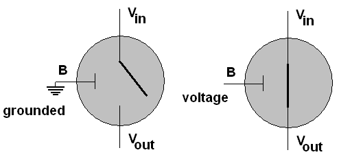
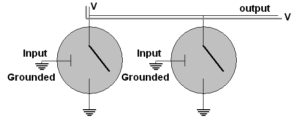
I will diagram a transistor as a gray circle.  A transistor has three connections, a base, B, an emitter, V_in, and a collector, V_out.  The base acts as a switch:  If the base is grounded, the emitter is not connected to the collector.  The symbol for ground is shown connected to the base in the left diagram above.  If a voltage is applied to the base, an electrical connection is enabled between emitter and collector.  Hence a transistor has two states, switched on or off.


Circuits are set up with a voltage source and opportunities for wires to be grounded.  The circuits are set up (with electrical resistances - we will skip elaborate physics) so if a wire is connected to ground, it is grounded, whether is is also connected to a voltage source or not. 

V_in is always connected to a source that might have a voltage on it or be grounded or be disconnected, while V_out may either be disconnected or grounded (but it does not have a voltage attached).  The standard ground symbol is shown at the bottom of each diagram below.  A capital V is used to mean a consistent voltage source.  A connection of the output to voltage or ground is shown by a gray path.

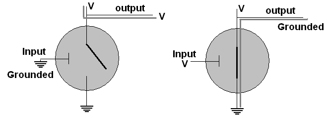
In the simplest situation, V_in is definitely connected to a voltage source and also to an output wire.  V_out is grounded.  In this case the state of the base is the only thing variable.  As the right diagram shows, if the base has a voltage, the emitter circuit is connected, and ground at V_out is connected to the output through V_in, so the output becomes grounded.  If the base does not have a voltage, as in the left diagram, the connection between the output and ground is broken, and the output is just connected to the regular voltage source, resulting in a voltage on the output wire.

Possibilities in the Figure

The circuit provides an output that is the opposite of the input.  If we associate voltage with 1 and grounded with 0, we get the NOT truth table!  The NOT operation takes only a single transistor.  

Possibilities in the Figure

We can connect two transistors in series as shown and use both bases as inputs.  

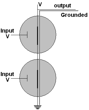
Only when both inputs have voltage, as shown, is there a connection between ground and the output.  If either input were grounded, the connection of ground and output would broken, and the output would hold voltage rather than being drawn to the ground state.  Hence if we call the inputs A and B and the output X, we get what is called a NAND gate.

Truth Table for a Nand gate:

This the truth table for (AB)', NOT  (A AND B), and the combination is commonly abbreviated, NAND.  

We can also connect two transistors in parallel as shown, still using both bases as inputs feeding one output.  

The only way to avoid a connection between the output and ground is to have both inputs grounded, as shown above, resulting in voltage at the output.  If at least one input has voltage, the output becomes connected to ground.  Hence if we call the inputs A and B and the output X, we get what is called a NOR gate:

Truth Table for a Nor gate:

This is the truth table for NOT (A  OR B), commonly abbreviated as NOR.  

To turn a Nor circuit into an Or circuit, a further NOT operation is needed on the output, requiring one more transistor.  Similarly you can convert a Nand to And with an extra transistor.  

In circuit diagrams, the details of the combinations of transistors, voltages and grounds needed for the different Boolean operations discussed above is hidden, or abstracted away.  The operations are given special, more simple symbols:


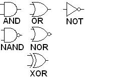
The inputs are assumed to come into the wires on the left and the output go out from the wire on the right.  All the gates that involve "NOT" have a small circle where the NOT operation would take place.

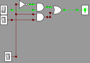
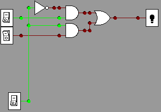
For example the Boolean expression A(B+C) corresponds to the circuit diagram



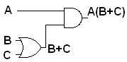
Each input is assumed to correspond to a voltage on a labeled wire, usually coming from the left.  These wires feed gates with result wires coming out of them.   As long as each wire ends up going to the left, and not looping, each wire corresponds directly to one Boolean expression.  Following the wires, putting the symbolic result as a label on each one in turn, eventually leads us to an output. 

There is a direct correspondence between the intermediate wires (like the one labeled B+C above),  their logical labels, and intermediate columns you should put in a truth table when looking to figure out the table for a boolean expression involving multiple operations.

These are sequential circuits.  Circuits with loops in them are also important, but more complicated.  They are call combinatorial circuits and will be briefly discussed later.

We will mostly work in terms of AND, OR, and NOT, because of their familiarity, though NAND and NOR are used more in actual engineering practice, since they require fewer transistors in a circuit.

By putting more than two transistors in series or parallel, NAND and NOR gates with more than two inputs can be constructed, hence with a further transistor for each added input, multi-input AND and OR gates can be constructed.  The same AND and OR gate symbols are used in these cases, except more input wires are allowed. 

Gates Applet (vid N5D)

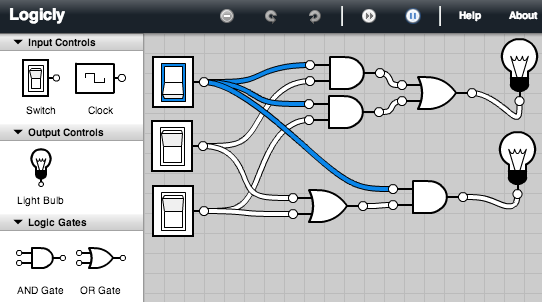
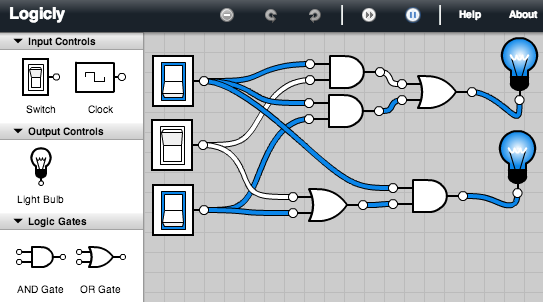
This section was originally developed with an old circuit simulator that is no longer useful.  The idea is the same as http://logic.ly/download/.  You can get a free 30-day download or just run the demo version in your browser.  It uses about the same symbols, dragging them into position, dragging between terminals to create wires.  In the new version there is no button to delete a wire:  just click in the middle of the wire and press the delete key.  In this version simulation is automatically running.  In the newer version there are no intermediate terminals:  all wires go from and output terminal to an input terminal.   Several wires can start from the same output terminal. Clicking on Help pretty well describes the use of the application.  I wish I had this one when I first made the diagrams and videos!

Watch the gatesApplet video, as I select and move components, connect them with wires, run the circuit and change input values  Try similar things with the Logicly simulator. The video ends with a demonstration discussed in the next paragraph (though using the old simlator images). 

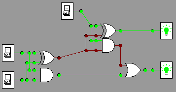
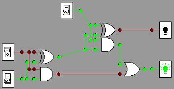
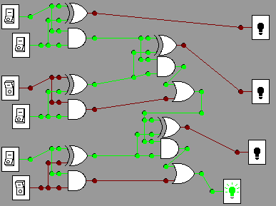
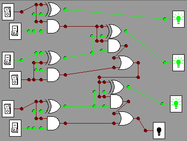
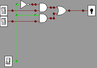
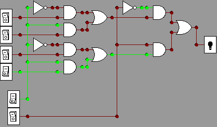
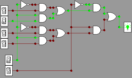
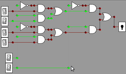
The following circuit tests the distributive property, AB+AC = A(B+C), assuming the inputs are labeled down from the top A, B, C.  The circuit has outputs for both sides of the identity originating from the same inputs, that fork two ways.  (This is fine, an input can feed several gates.)  No matter how you manipulate the three switches to give all the possible inputs, the two outputs always match.  This is illustrated for inputs 1, 0, 0 and for 1, 0, 1, where we use 1 to denote a switch with voltage, denoted in the simulator with a blue rectangle around the switch.  The convention is that wires only go from the output of a component to the input of another, with only one wire going to any input terminal.

Finding a Boolean Expression for a truth table (vid N5E)

In the introduction, I mentioned that we want to be able to convert between all the representations: circuit, boolean expression, and truth table.  We have discussed the direct translation between Boolean expressions and circuits, and we have shown how to convert a Boolean expression into a truth table.  The only direction missing now is from truth table to Boolean expression.

Below is a truth table for an output X.  It is totally specified by the truth table, without first being given by a Boolean expression.  To find a Boolean expression that does correspond to the output X, first locate a 1 in the column for X.  The final row is an example.  This is true when we have the exact input values in the row: A is true and B is true and C is true.  That is a simple statement to translate into boolean symbolism:  ABC.  Another row where X is one is the third from the bottom, where A is true and B is not true and C is true.  Another way to put this is A is true and (not B) is true and C is true.  Again, this easily translates into a Boolean expression:  AB'C.  The chart below traces out the sequence of steps, including for the second row :

A B C  X              Example
0 0 0  0
0 0 1  1
0 1 0  0
0 1 1  0
1 0 0  0
1 0 1  1
1 1 0  0
1 1 1  1  <- First find an expression producing this 1 and = 0 everywhere else

A B C  X
0 0 0  0
0 0 1  1
0 1 0  0
0 1 1  0
1 0 0  0
1 0 1  1  <- Find expression producing this 1 and = 0 everywhere else
1 1 0  0
1 1 1  1  ABC

A B C  X
0 0 0  0
0 0 1  1 <- Find expression producing this 1 and = 0 everywhere else
0 1 0  0
0 1 1  0
1 0 0  0
1 0 1  1  AB'C  
1 1 0  0
1 1 1  1  ABC

A B C  X
0 0 0  0
0 0 1  1 A'B'C
0 1 0  0
0 1 1  0
1 0 0  0
1 0 1  1  AB'C  
1 1 0  0
1 1 1  1  ABC

We have expressions = 1 ONLY in each individual place X is 1.  To get X, which is 1 with any of these inputs, combine with the OR operation:  
X = A'B'C + AB'C + ABC  

Simplifying Boolean Algebra

A circuit could certainly be made for X, but it would be easier with a simplification.  One advantage of Boolean algebra is that it is easy to manipulate algebraically, for instance using the rules of Boolean Algebra discussed earlier.  I will not hold you responsible for this, but it will shorten some answers, and hence prove to be convenient! 

Focus on the last two terms:
A'B'C + (AB'C + ABC)
= A'B'C + AC(B'+B)   distributive rule (factoring out A and C
= A'B'C + AC(1)      complement rule for OR
= A'B'C + AC         identity rule

One general rule that is easy to check that was not in the earlier rules is
A + A = A
In general, this means any expression can be replaced by two ORed copies of the same expression.  In particular the one copy of AB'C in the middle of the expression for X can be replaced by two copies ORed:

X = A'B'C + AB'C + ABC
= A'B'C + AB'C + AB'C + ABC      adding a second ORed copy of AB'C
= (A'B'C + AB'C) + (AB'C + ABC)  associating parts usefully
= (A'B'C + AB'C) + AC                         using the result above for the last two terms

Just as we showed AB'C + ABC = AC, we can rework the first two terms:

(A'B'C + AB'C) + AC
= (A' + A)B'C  + AC
= (1)B'C       + AC     
=    B'C + AC

The general pattern that simplifies is when all but one factor matches in two terms:  then the non matching factor (negated in one term and not negated in the other) can be completely removed and leave only one term with the remaining common factors.  Symbolically, if X stands for all the matching factors and Y is the one non matching factor then XY + XY' = X.

A Further Example: English to Truth Table to Boolean Expression

Find a truth table for the Boolean expression that is true when all three inputs (A, B, C) are the same  (call this X initially).  Then find the Boolean expression in terms of A, B, and C. 

A B C  X
0 0 0  ?
0 0 1  ?
0 1 0  ?
0 1 1  ?
1 0 0  ?
1 0 1  ?
1 1 0  ?
1 1 1  ? 

Coming up with a completed truth table involves an inital translation from English:

A B C  X
0 0 0  1
0 0 1  0
0 1 0  0
0 1 1  0
1 0 0  0
1 0 1  0
1 1 0  0
1 1 1  1  

Now what to get a Boolean expression?

A B C  X
0 0 0  1  <- First find AN expression matching this 1 and = 0 everywhere else
0 0 1  0
0 1 0  0
0 1 1  0
1 0 0  0
1 0 1  0
1 1 0  0
1 1 1  1

A B C  X
0 0 0  1  A'B'C'
0 0 1  0
0 1 0  0
0 1 1  0
1 0 0  0
1 0 1  0
1 1 0  0
1 1 1  1 <- Then find AN expression matching this 1 and = 0 everywhere else


A B C  X
0 0 0  1  A'B'C'
0 0 1  0
0 1 0  0
0 1 1  0
1 0 0  0
1 0 1  0
1 1 0  0
1 1 1  1 ABC

Then what?

Combine with OR:

X = A'B'C' + ABC

A common student error is to skip the last step, and not combine, but you are looking for a description of a single output, so your result must be a single expression!

Addition in Computer Circuits (vid N5F)

OK so we can convert logical operations to hardware.  In all our logical operations, however, we did not see normal arithmetic, but we want to be able to do that on a computer!  Since we are using two state circuits we will do binary arithmetic.  Start as simply as possible.  If we stick to 1 bit additions, there are not many choices:

 0   0   1   1
+0  +1  +0  +1
__  __  __  __
 0   1   1  10

The complication is the carry in the last case.  It means we need to keep track of two binary outputs which we will call sum (the 1's bit) and carry (the carry bit).  All the data is 0's and 1's, so we can write a complete table:

Table for sum and carry in binary addition, A+ B

We are thinking of arithmetic, but see the format of the table - it is in the format of a truth table!
You may recognize both the outputs:  carry is AND and sum is XOR.  

If you wish to avoid the XOR symbolism, you can calculate an equivalent expression in terms of AND, OR, and NOT, as we can for a truth table.  Applying the technique just introduced for finding a Boolean expression from a truth table, you find:
A XOR B = AB' + A'B

This is a half adder circuit.

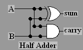
The video animates this circuit.  If you like you can construct and test the circuit for yourself in the gates applet,

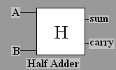
To understand more complicated circuits it is useful to give a simpler symbol for repeatedly used circuits.  We will use the half adder several times in more complicated situations, and will give the half adder its own symbol



When you do addition using place value with two multi-digit numbers, you actually have to add three digits together at a time in general:  a digit from each number, and a possible carry from the previous place.  An example as you might have written it in primary school to add 5147 and 7689:

  1 11   carries
   5147  decimal numeral
 + 7689  decimal numeral
  _____
= 12836   

If you are adding multi bit binary numerals, that means adding three inputs that can be 0 or 1, with a sum at most 3, still only needing 2 bits of output.  

   111   carries
    011  binary numeral
 +  111  binary numeral
  _____
=  1010

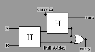
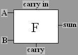
We can put two half adders together with one extra OR gate to create a full adder, which adds three single bit inputs, as illustrated below in terms of the just-introduced half adder symbol.  If we label the three inputs A, B, and "carry in", then we can start adding A and B with a half adder.  The sum output can be added to the carry in with another half adder to produce the final sum bit.  Both half adders have a carry bit.  If either one produces a carry, then there is a carry in the final answer, so the carry bits need to go through an OR gate to procuce the final carry.



Recreating this in the gates applet is shown in the video, and also below in pictures.  The most significant output bit (carry) in at the bottom.  You could also create your own and test it in the gates applet, but the circuits are getting more complicated to reproduce by hand!
.  1+1+1 =11

  1+0+1=10
The full adder, too, can be used in more complicated circuits, so we will give it its own symbol:

 

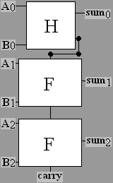
Once you have full adders you can chain them together to create a multi-bit adder.  For example, a circuit to add two three-bit numbers could get inputs A₂, A₁, A₀, and B₂, B₁, B₀, where the subscripts indicate the power to which 2 is raised in the binary place value.  The result produces three sum bits for 2 raised to powers 0, 1, and 2, and a further bit for the final carry (representing 2³). The addition in the lowest order bit has no carry in, so only a half adder is needed:



Recreating this in the gates applet is shown below in pictures, and is simulated in action in the video.  For example, consider these two calculations:

 11     
 011   010
+101  +101
____  ____  
1000   111

The pictures below show these two calculations in a circuit, with the more significant bits in both the input and output are lower down in the diagram.  The top summands in the manual calculations above correspond tothe leftmost column of switches, and the bottom summmands reappear slightly to the right. 

  011+101=1000

  010+101 = 111

Multiplexers (vid N5G)

A multiplexer chooses one of several data lines.  In an n-bit multiplexer input consists of 2ⁿ data lines and  n control lines for some positive value of n.  There is one output line.  The n control lines have 2ⁿ possible states and hence they can be wired to determine which of 2ⁿdata lines should go to the one output line.  For example if the control lines hold a memory address, multiplexers can be used to fetch the data fromthe proper source.  The simplest version to illustrate is a 1-bit multiplexer shown below.  It shows 2 data line and 1 control line (the control line can choose between two states).  In the pictures below data bits are indexed by 0 at the top, 1 below, and the one control line at the bottom chooses between them.   For example, in the first picture the control line is off (0), so the input with index 0 (the upper one) has its state (on, 1) transmitted through to the output wire, lighting the light.
d0=1, d1=0, control choosing d0 = 1
d0=1, d1=0, control choosing d1 = 0
d0=0, d1=0, control choosing d1

The pictures below, and also the Multipler video show a 2-bit mutiplexer, with 4 data lines and 2 control lines.  (Do you see that it is composed of three of the simpler multiplexers?)  In general there could be 2ⁿ  data lines and n control lines.  The data lines in the picture are numbered 00 through 11 from top to bottom.  The top control line has the less significant bit.

d00=0, d01=0, d10=0, d11=1, control choosing d01 = 0

d00=0, d01=1, d10=0, d11=0, control choosing d01 = 1

A demultiplexer does the reverse:  n control lines and one data input line deliver the input value to one of 2ⁿ output data lines.

Multiplexers are needed to fetch data from one of many memory addresses.  Instructions must be fetched, using the IP address to feed the control lines.  We need to get data into a register, like the accumulator in Pip, using the address byte in an instruction to feed the control lines.  Also Demultiplexers are needed for the reverse:  getting data from the accumulator to one of many memory addresses.  Multiplexers can also be used inside a CPU to get the result from a specified operation code:  The computer actually works out all possible operations at the same time, feeding data lines into a multiplexer;  the op code feeds the control lines of this multiplexer to pick the result associated with the right op code.

Latch Circuit (vid N5H)

We have only considered sequential circuits - signals flow through and nothing is kept.  We need a combinatorial circuit, one with a loop in it, to have memory.  Loops in circuits can get tricky.

A latch can remember a value.  We examine it in steps.



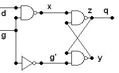
It has two main direct inputs d, the data value, and g, which is 1 as we shall see when the circuit should get the data.  Note the two lines feeding back from the nand outputs y and z.  Also z flows to the final circuit output q.  The three nand gates correspond to Boolean relationships x = (dg)'; z = (xy)'; y = (g'z)'  

If g is 1, then g' is 0, and this simplifies to x = (d1)' = d'; y = (0z)' = (0)' = 1, so z = (d'1)' = (d')' = d, and q = z:  that means the value of d is transmitted to the output, whatever d is, and however it changes over time.



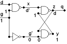
On the other hand, if g is 0, then g' is 1, and it is more complicated, and we must take the old value of z into account:  call that old value q, so q = z. Then x = (0d)' = 1, and d has no further effect.  y = (1q)' = q' which then circles around to make z = (1q')' = q, which is what it was before, so the loop maintains its old value of z (and also its value of y similarly), independent of how d is changed!  



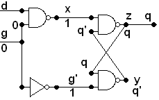
It is not quite that simple if you view the latch video.  If you try to recreate it and run it in a simulator with lower input g = 1, you can switch the upper input d and have it behave as expected.  However if you change d to 1 and then change g to 0, then depending on your Java implementation for the applet, you could see the circuit flash continuously, back and forth between the two pictures below:

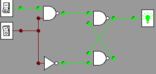
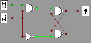
That transition of g from 1 to 0 is a problem.  This is a timing issue.  See the slight alteration below.  See that two extra NOT gates are inserted.  In a static logical state they cancel each other out, but they change the timing when the signal from g alters and splits.  Now runing a simulation works, if you start from a stable state, with any sequence of input data, and it should work (hopefully in whatever version of Java your browser is using). 

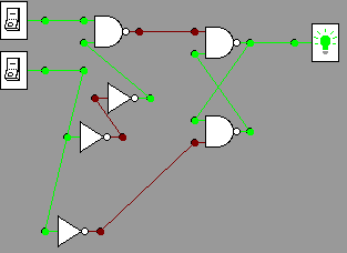With g=1, data 1 passes though.  If data were switched to 0, output would go to 0.

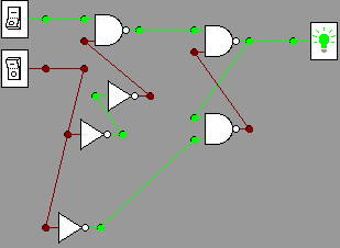  g to 0, keep output 1

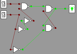  g at 0, data switched to 0, but output still 1

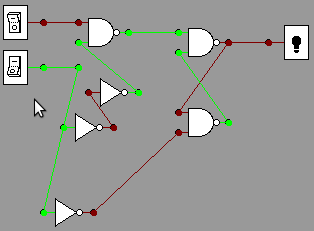  g to 1, output matched data, 0

 When the lower input (g) is 1, the output changes with the upper input (d).  When g is changed to 0, the last output is remembered, no matter what you do later to d. 

This example indicates the importance of timing.  We have left out a discussion of the regular alternating clock signal that is used to synchronize and stabilize outputs.  A deeper examination of circuits would include a clock.


See the gates homework.

Very Large Scale Integration in Circuits (VLSI) (vid N5I)

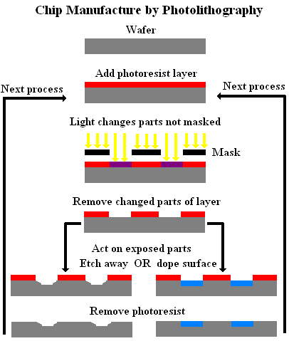
For much more detail (going far beyond this course!), see  VLSI or this extensive and technical pdf. 

Conclusion (vid N6)

So we have gotten as far down to basics as we are going to in this class.  (Below this is chemistry and physics!)  We have described some of the most important hardware used in creating a computer, seen how millions of components can be put together efficiently to create a machine with its machine language, and some of the major points in the translation between machine language and a high level language.  

There is much more to study.  Here are a few examples:

• Comp 264, Computer Systems, covers what lies under high level languages in much greater depth.
  

• A sequence of programming courses, starting with Comp 170, show ideas needed for more sophisticated programs to solve much larger problems.

• There are a great many topics in computer science beyond programming, addressed in upper level courses:  

  • networking and security,

  • devising algorithms for handling all kinds of enormous collections of data,
    
    

  • organizing and accessing enormous databases
    

  • getting many processors and many computers to work together effectively on enormous problems,

  • dealing with the many legal and ethical issues around computing,

  • approximating human intelligence (so far only in specialized ways),

  • and finally finding the limits of computing - it cannot solve all problems.  

There is much more to learn and apply to the pressing problems of today and tomorrow!   We live in the information age!   Will you be a leader in it?

We have been dealing with the current practical model, with Boolean electical components on a chip.  Completely different approaches are being researched and may have practical  application in the future: optical computers, quantum computers, DNA computers, ....